Chapter 3Linear transformations and matrices

Published Aug 7, 2016

Updated Jan 22, 2024

Text adaptation by Kurt Bruns

Text adaptation by River Way

"Unfortunately, no one can be told what the Matrix is. You have to see it for yourself."
- Morpheus

If I had to choose just one topic that makes all of the others in linear algebra start to click, it would be this one. We'll be learning about the idea of a linear transformation, and its relation to matrices. For this chapter, the focus will simply be on what these linear transformations look like in the case of two-dimensions, and how they relate to the idea of matrix-vector multiplication.

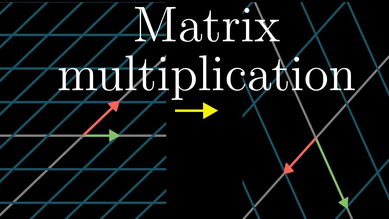
In particular, I want to show you a way to think about matrix multiplication that doesn't rely on memorization.

Transformations Are Functions

To start, let's parse this term: "Linear transformation". Transformation is essentially a fancy word for function; it's something that takes in inputs, and spit out some output for each one.

Specifically, in the context of linear algebra, we think about transformations that take in some vector, and spit out another vector.

So why use the word "transformation" instead of "function" if they mean the same thing? It's to be suggestive of a certain way to visualize this input-output relation. Rather than trying to use something like a graph, which really only works in the case of functions that take in one or two numbers and output a number, a great way to understand functions of vectors is to use movement.

'Transformation' suggests movement!

If a transformation takes some input vector to some output vector, we imagine that input vector moving to the output vector.

To understand the transformation as a whole, we imagine every possible vector move to its corresponding output vector.

Vectors As Points

It gets very crowded to think about all vectors all at once, each as an arrow. So let's think of each vector not as an arrow, but as a single point: the point where its tip sits. That way, to think about a transformation taking every possible input vector to its corresponding output vector, we watch every point in space move to some other point.

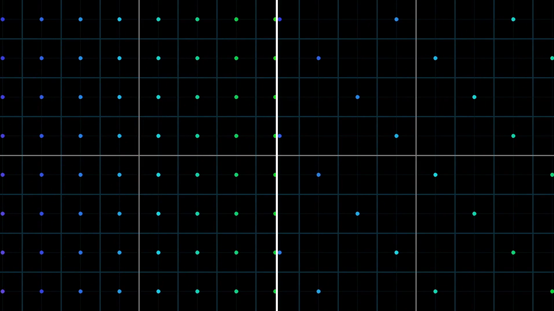
In the case of transformations in two dimensions, to get a better feel for the shape of a transformation, I like to do this with all the points on an infinite grid. It can also be helpful to keep a static copy of the grid in the background, just to help keep track of where everything ends up relative to where it starts.

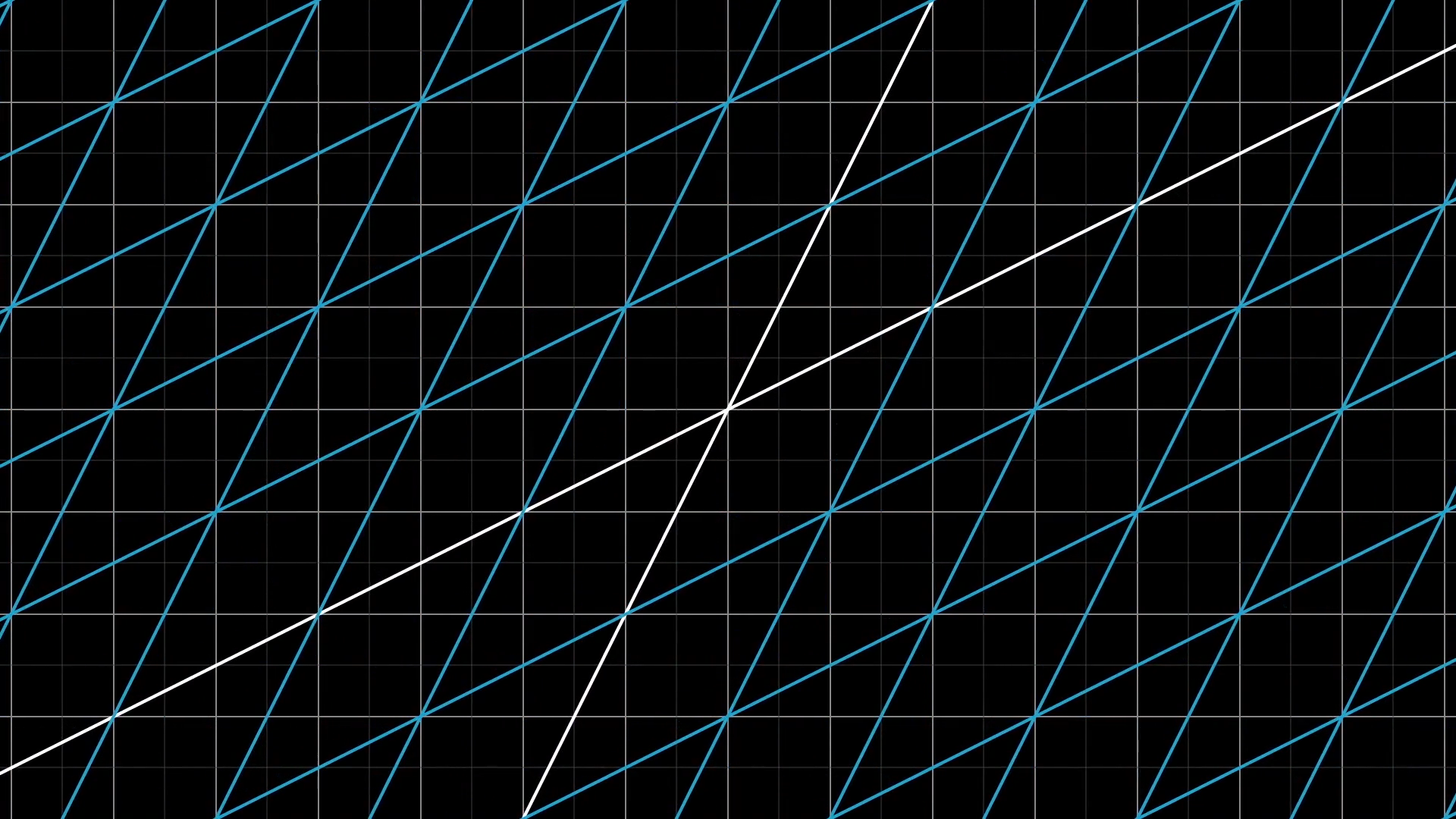
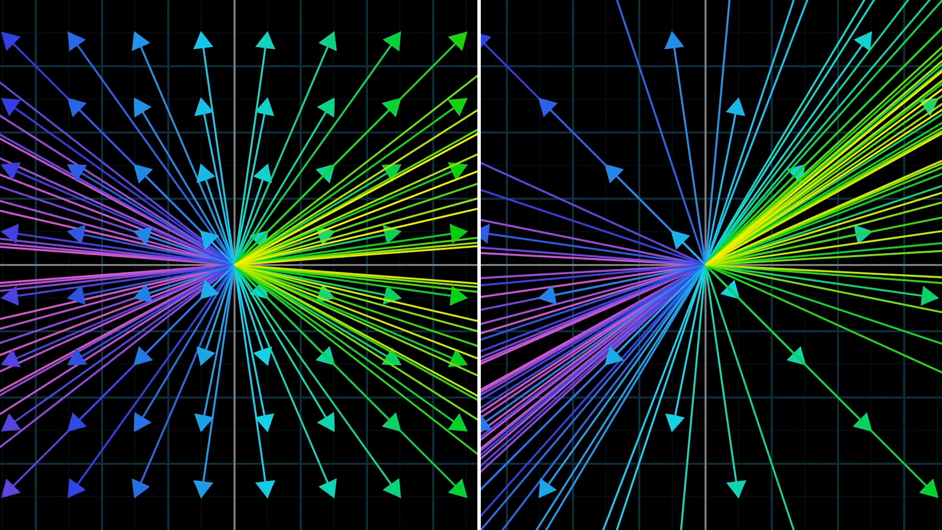
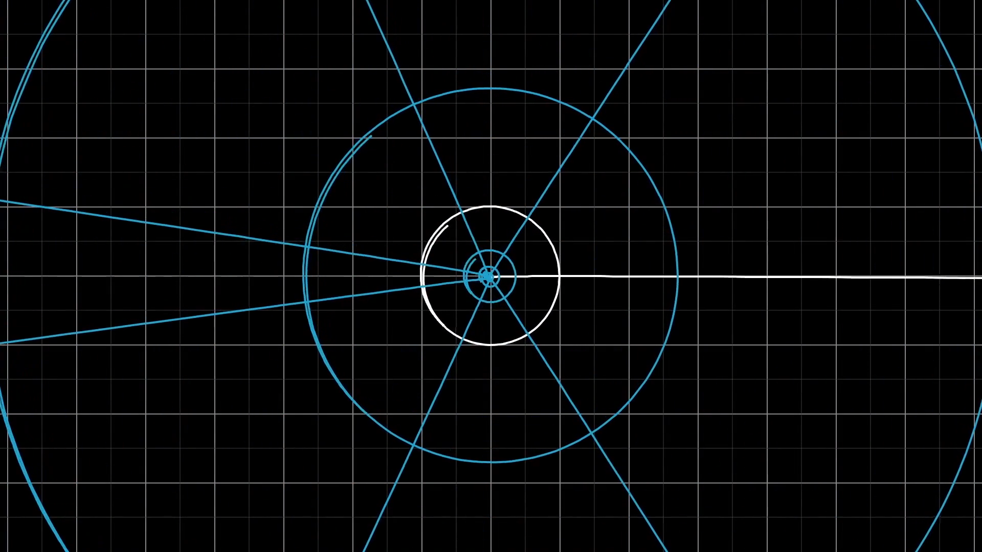
Visualizing functions with 2d inputs and 2d outputs like this can be beautiful, and it's often difficult to communicate the idea on a static medium like a blackboard. Here are couple more particularly pretty examples of such functions.

What makes a transformation "linear"?

As you can imagine, though, arbitrary transformations can look pretty complicated, but luckily linear algebra limits itself to a special type of transformation that's easier to understand called Linear transformations. Visually speaking, a transformation is "linear" if it has two properties: all lines must remain lines, without getting curved, and the origin must remain fixed in place.

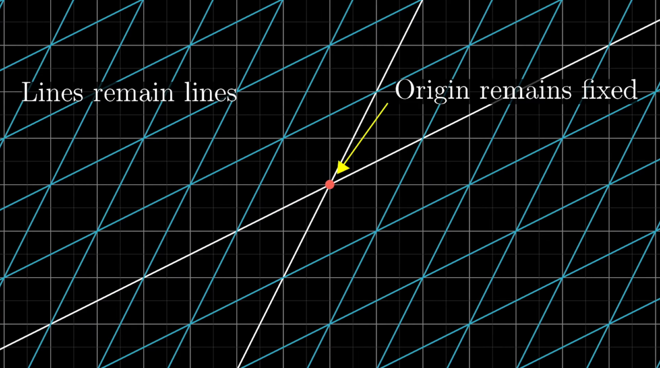
For example, this right here would not be a linear transform, since the lines get all curvy.

And this one would not be a linear transformation because the origin moves.

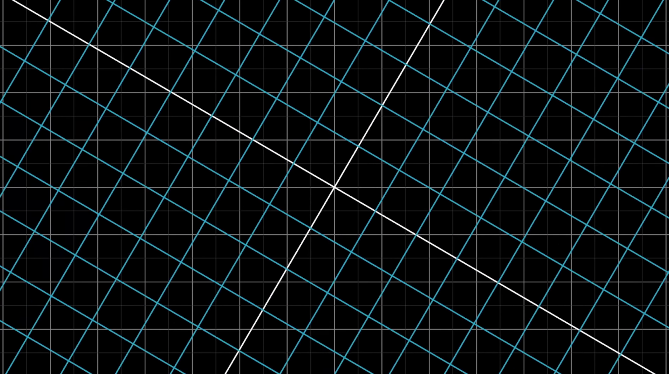
This one here fixes the origin, and it might look like it keeps lines straight, but that's just because I'm only showing horizontal and vertical grid lines.

When you see what it does to a diagonal line, it becomes clear that it's not a linear transformation at all, since it turns that line all curvy.

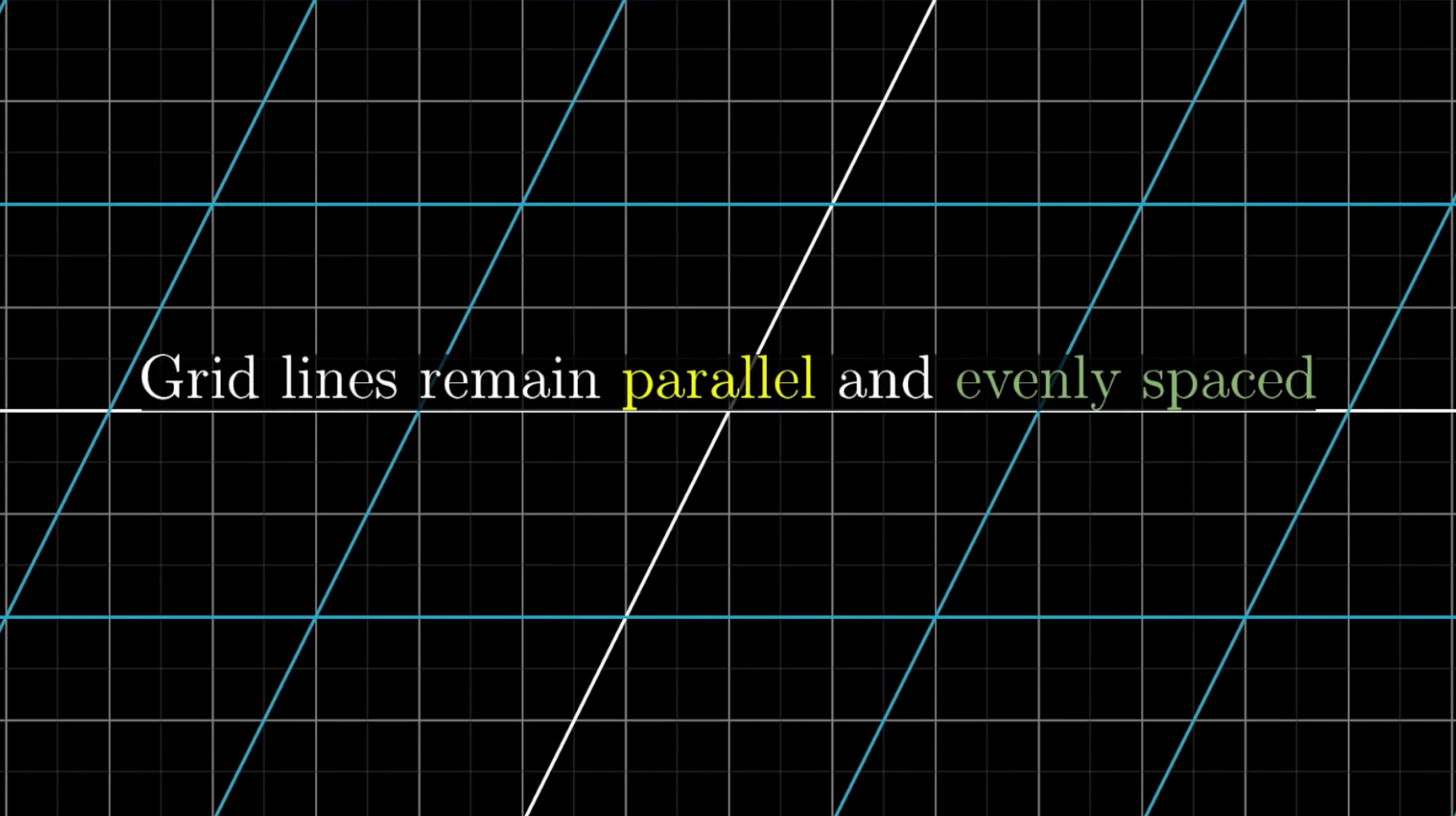
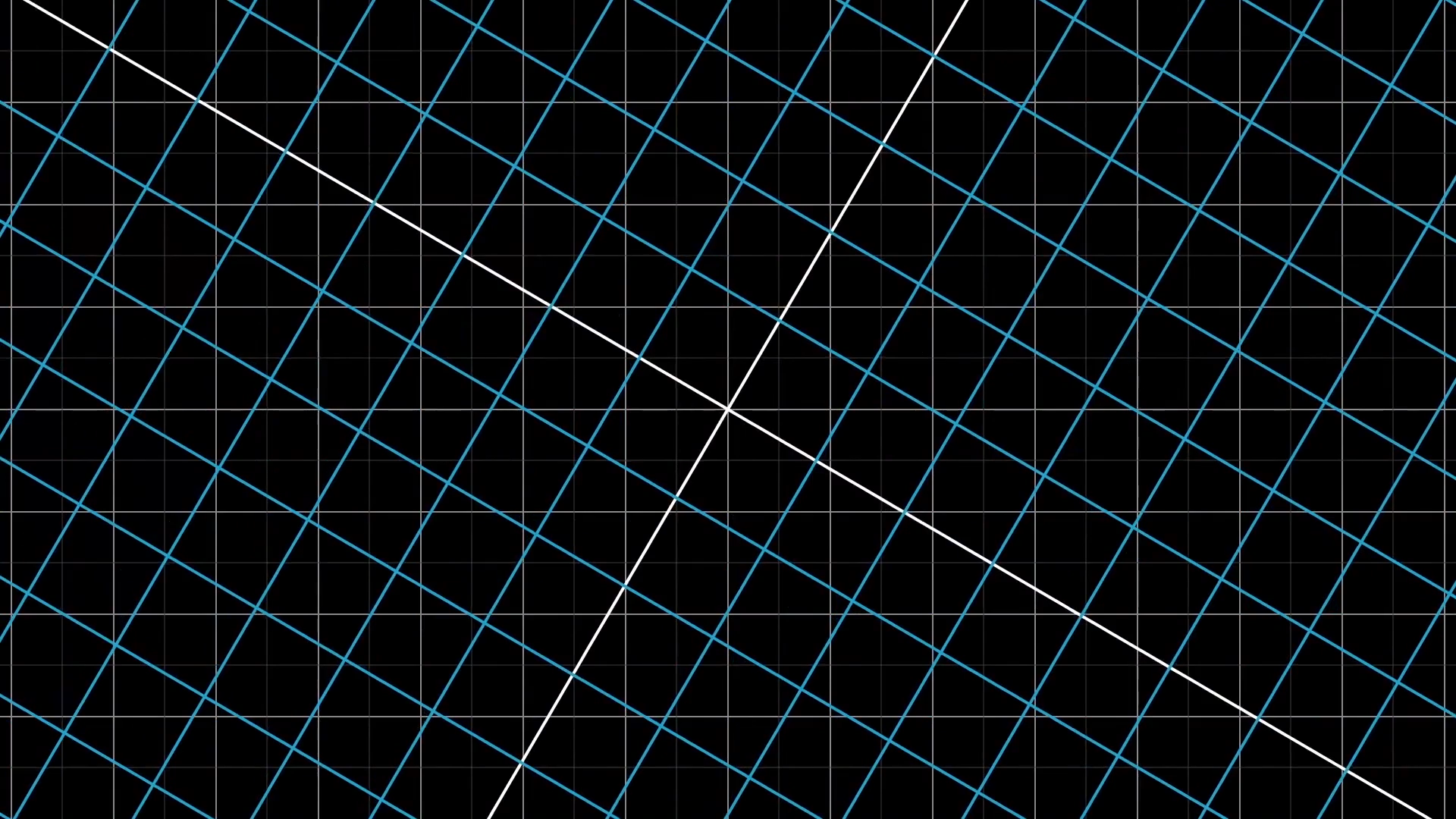
In general you should think of linear transformations as keeping grid lines parallel and evenly spaced, although they might change the angles between perpendicular grid lines. Some linear transformations are simple to think about, like rotations about the origin. Others are a little trickier to describe with words.

Some linear transformations are simple to think about, like rotations about the origin.

This linear transformation rotates XX about the origin.

Others, as we will see later, are a little trickier to describe with words.

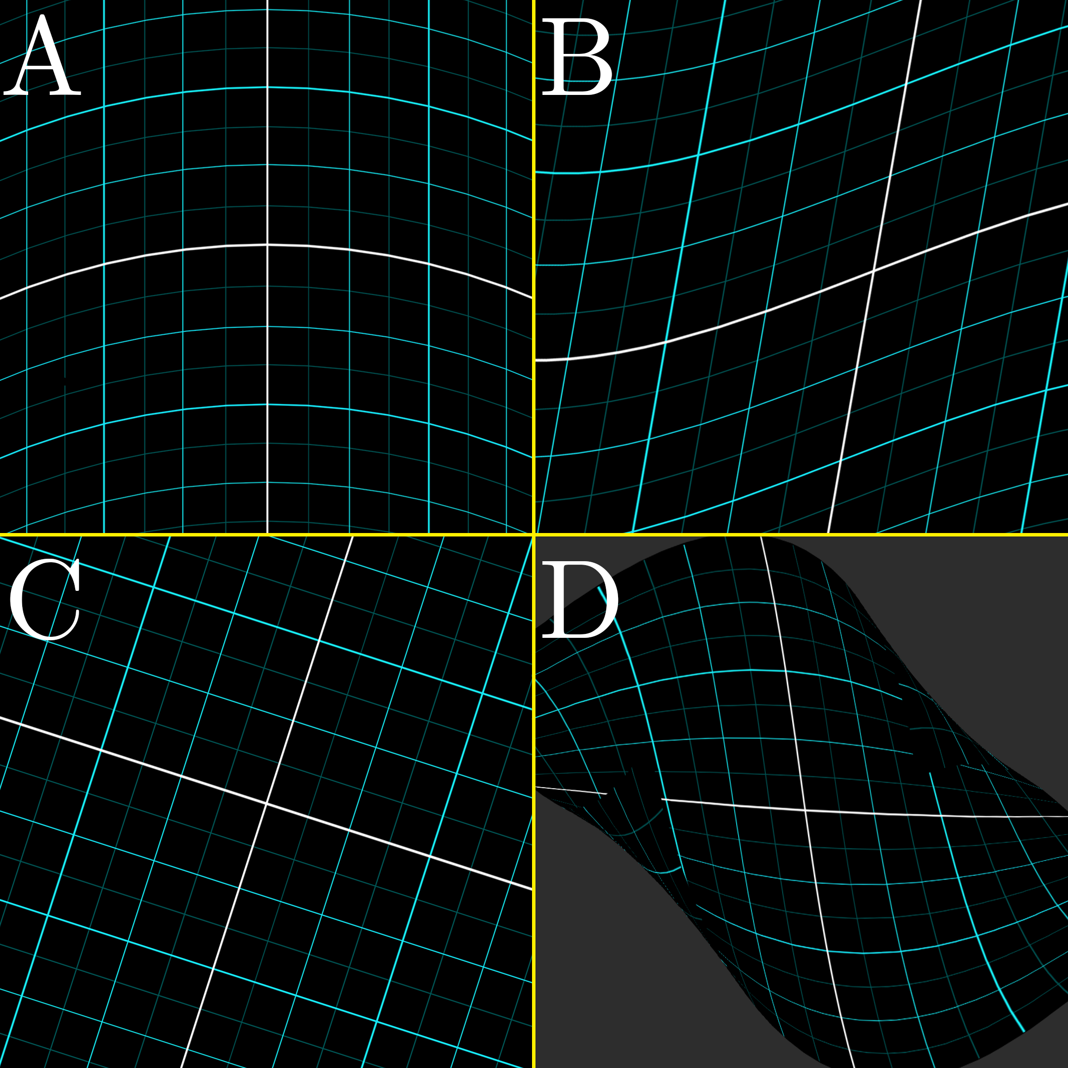
Which of the transformations in the image below are linear?

Matrices

How do you think you could do these transformations numerically? If you were, say, programming some animations to make a video teaching the topic, what formula do you give the computer so that if you give it the coordinates of a vector, it can tell you the coordinates of where that vector lands.

How would you describe one of these transformations using a formula?

It turns out, you only need to record where the two basis vectors i-hat and j-hat go, and everything else will follow.

For example, consider the vector $\vec{\mathbf{v}}$ with coordinates $\begin{bmatrix}-1\\2\end{bmatrix}$ , meaning it is equal to $-1\hat{\imath} + 2\hat{\jmath}$ .

If we play some transformation, and follow where all three of these vectors go, the property that grid lines remain parallel and evenly spaced has a really important consequence: the place where v lands will be (-1) times the vector where i hat landed, plus 2 times the vector where j hat landed.

In other words, it started off as a certain linear combination of i hat and j hat, and it ended up at that same linear combination of where those two vectors landed.

$L(\vec{\mathbf{v}})= -1 \begin{bmatrix}1\\-2\end{bmatrix}+2 \begin{bmatrix}\:3\:\\0\end{bmatrix}$

Now, given that I'm actually showing you the full transformation, you could have just looked to see that v has coordinates [5, 2], but the cool part here is that this gives us a technique to deduce where the vector lands without needing to watch the transformation.

This is a good point to pause and ponder, because it's pretty important.

Given a transformation with the effect $\hat{\imath}\to\begin{bmatrix}-1\\1\end{bmatrix}$ and $\hat{\jmath}\to\begin{bmatrix}-2\\-1\end{bmatrix}$ , where will it take the input $\vec{\mathbf{v}} = \begin{bmatrix}-3\\-1\end{bmatrix}$ ?

$\begin{bmatrix}5\\-2\end{bmatrix}$

$\begin{bmatrix}4\\-1\end{bmatrix}$

$\begin{bmatrix}-5\\2\end{bmatrix}$

$\begin{bmatrix}5\\1\end{bmatrix}$

So long as we have a record of where i hat and j hat land, this technique works for any vector vector that is passed to the transformation function.

Many vectors transformed by the function that sends i hat to $\begin{bmatrix}1\\-2\end{bmatrix}$ and j hat to $\begin{bmatrix}3\\0\end{bmatrix}$ .

Writing the vector with more general coordinates, $x$ and $y$ : It will land on $x$ times the vector where i hat lands, [1, -2], plus y time the vector where j hat lands, [3, 0].

L(\vec{\mathbf{v}}) = x\left[\begin{array}{c}1 \\-2\end{array}\right]+y\begin{bmatrix}\:3\:\\0\end{bmatrix}

Carrying out that sum, we see that it lands on [1x + 3y, -2x + 0y]. I give you any vector, and you can tell where it lands using this formula.

L(\vec{\mathbf{v}}) = \begin{bmatrix}1x + 3y \\ -2x + 0y \: \end{bmatrix}

What all of this is saying is that the two-dimensional linear transformation is completely described by just four numbers: The two coordinates for where i hat lands, and the two coordinates for where j hat lands. Isn't that cool?

It's common to package these four numbers into a 2x2 grid of numbers, called a “2x2 matrix”, where you can interpret the columns as the two special vectors where i hat and j hat land.

If you're given a 2x2 matrix describing a linear transformation, and a specific vector, and you want to know where the linear transformation takes that vector, you take the coordinates of that vector, multiply them by the corresponding column of the matrix, then add together what you get. This corresponds with the idea of adding scaled versions of our new basis vectors.

CurrentProgress

Current progress is here

This is all the information we need to apply the transformation to an input vector.

For example, let's bring back our vector $\overrightarrow{\mathbf{v}} = \begin{bmatrix}-1\\2\end{bmatrix}$ from earlier, and consider the linear transformation we were looking at previously, which looks like this.

By comparing the outputs of the transformation with the faint static grid in the background, we can see that the transformation has taken $\overrightarrow{\mathbf{v}}$ to the output $\begin{bmatrix}5\\2\end{bmatrix}$ .

But suppose you were just given the data describing what the transformation does to $\color{green} \hat{\imath}$ and $\color{red} \hat{\jmath}$ , and you wanted to compute where $\overrightarrow{\mathbf{v}}$ goes without looking at pre-created picture. How would you do it?

For the transformation shown above, here's the relevant data.

L({\color{green} \hat{\imath}}) = \begin{bmatrix}1\\-2\end{bmatrix} \qquad L({\color{red} \hat{\jmath}}) = \begin{bmatrix}3\\0\end{bmatrix}

Using those four numbers, here's how you could compute where $\overrightarrow{\mathbf{v}} = \begin{bmatrix}-1\\2\end{bmatrix}$ will go.

\begin{align*} L(\overrightarrow{\mathbf{v}}) &= L(-1 {\color{green}\hat{\imath}} + 2 {\color{red}\hat{\jmath}}) \\\\ &= -1 \cdot L({\color{green}\hat{\imath}}) + 2 \cdot L({\color{red}\hat{\jmath}}) \\\\ &= -1 \cdot \begin{bmatrix}1\\-2\end{bmatrix} + 2 \cdot \begin{bmatrix}3\\0\end{bmatrix} \\\\ &= \begin{bmatrix}5\\2\end{bmatrix} \end{align*}

Reassuringly, this is the same value we found by just looking at the picture. But the important point is that to communicate what the transformation is without a picture, it's enough to simply give the coordinates of $L({\color{green}\hat{\imath}})$ and $L({\color{red}\hat{\jmath}})$ , and from there we can compute what happens to any other.

This is a good point to pause and ponder, because it's pretty important.

Given a transformation with the effect $\hat{\imath}\to\begin{bmatrix}3\\-2\end{bmatrix}$ and $\hat{\jmath}\to\begin{bmatrix}-1\\0\end{bmatrix}$ , where will it take the input $\begin{bmatrix}5\\-2\end{bmatrix}$ ?

$\begin{bmatrix}17\\-10\end{bmatrix}$

$\begin{bmatrix}13\\-12\end{bmatrix}$

$\begin{bmatrix}15\\-10\end{bmatrix}$

$\begin{bmatrix}15\\-2\end{bmatrix}$

Let's make this more general. Consider the same transformation we had above, the one whose behavior is entirely characterized by this data:

L({\color{green} \hat{\imath}}) = \begin{bmatrix}1\\-2\end{bmatrix} \qquad L({\color{red} \hat{\jmath}}) = \begin{bmatrix}3\\0\end{bmatrix}

Can you write a formula for what this does to a general vector $\begin{bmatrix}x\\ y\end{bmatrix}$ ? Really, take a moment to try write it out for yourself.

Your answer:

Our answer:

\color{black}\begin{bmatrix}x\\ y\end{bmatrix}\to x \color{green}\begin{bmatrix}1\\-2\end{bmatrix} \color{black}+y \color{red}\begin{bmatrix}3\\0\end{bmatrix} \color{black}= \begin{bmatrix} \color{green}1\color{black}x+\color{red}3\color{black}y \\ \color{green}-2\color{black}x+\color{red}0\color{black}y \end{bmatrix}

If you were able to get that, then congratulations, you just reinvented matrix vector multiplication.

You see, it's common to package these four numbers which characterize a given transformation into a $2\times 2$ grid of numbers, called a "2-by-2 matrix", where you can interpret the columns as the two special vectors where $\hat{\imath}$ and $\hat{\jmath}$ land.

``2\times 2\text{ Matrix''} \\\\ \begin{bmatrix} \color{green}1 & \color{red}3 \\ \color{green}-2 & \color{red}0 \end{bmatrix}

\begin{bmatrix} \color{green}3 & \color{red}2 \\ \color{green}-2 & \color{red}1 \end{bmatrix} \cdot \begin{bmatrix}5\\7\end{bmatrix} = 5\begin{bmatrix}\color{green}3\\ \color{green}-2\end{bmatrix} +7\begin{bmatrix}\color{red}2\\ \color{red}1\end{bmatrix} = \begin{bmatrix}29\\-3\end{bmatrix}

We can generalize this idea with a matrix that has variable entries:

\begin{bmatrix} \color{green}a & \color{red}b \\ \color{green}c & \color{red}d \end{bmatrix} \cdot \begin{bmatrix}x\\y\end{bmatrix} = x\begin{bmatrix}\color{green}a\\ \color{green}c\end{bmatrix} +y\begin{bmatrix}\color{red}b\\ \color{red}d\end{bmatrix} = \begin{bmatrix} \color{green}a\color{black}x+\color{red}b\color{black}y \\ \color{green}c\color{black}x+\color{red}d\color{black}y \end{bmatrix}

Remember that this all came from thinking about the columns as the transformed versions of your basis vectors. Then the result is the appropriate linear combination of those vectors.

Examples

Rotation

If we rotate all of space $90^\circ$ counterclockwise, then $\hat{\imath}$ lands on the $y$ -axis, and $\hat{\jmath}$ lands on the negative $x$ -axis.

To figure out what happens to any vector after a $90^\circ$ rotation, you can multiply its coordinates by this matrix.

\begin{bmatrix}0&-1\\1&0\end{bmatrix} \begin{bmatrix}x\\ y\end{bmatrix} =\begin{bmatrix}-y\\ x\end{bmatrix}

Shear

Here's a fun transformation with a special name, called a "shear". The $x$ -axis stays in place, but the $y$ -axis tilts $45^\circ$ to the right.

In it, $\hat{\imath}$ remains fixed, so the first column of the matrix is $\begin{bmatrix}1\\ 0\end{bmatrix}$ , but $\hat{\jmath}$ moves over to the coordinates $\begin{bmatrix}1\\ 1\end{bmatrix}$ , which becomes the second column of the matrix. Just like other matrices, we can multiply any vector to see how it transforms the vector:

\begin{bmatrix}1&1\\0&1\end{bmatrix} \begin{bmatrix}x\\ y\end{bmatrix} =\begin{bmatrix}x+y\\ y\end{bmatrix}

Transformation from a Matrix

If we are given a matrix, say $\begin{bmatrix}1 & 3\\ 2 & 1\end{bmatrix}$ , can you deduce what it's transformation looks like?

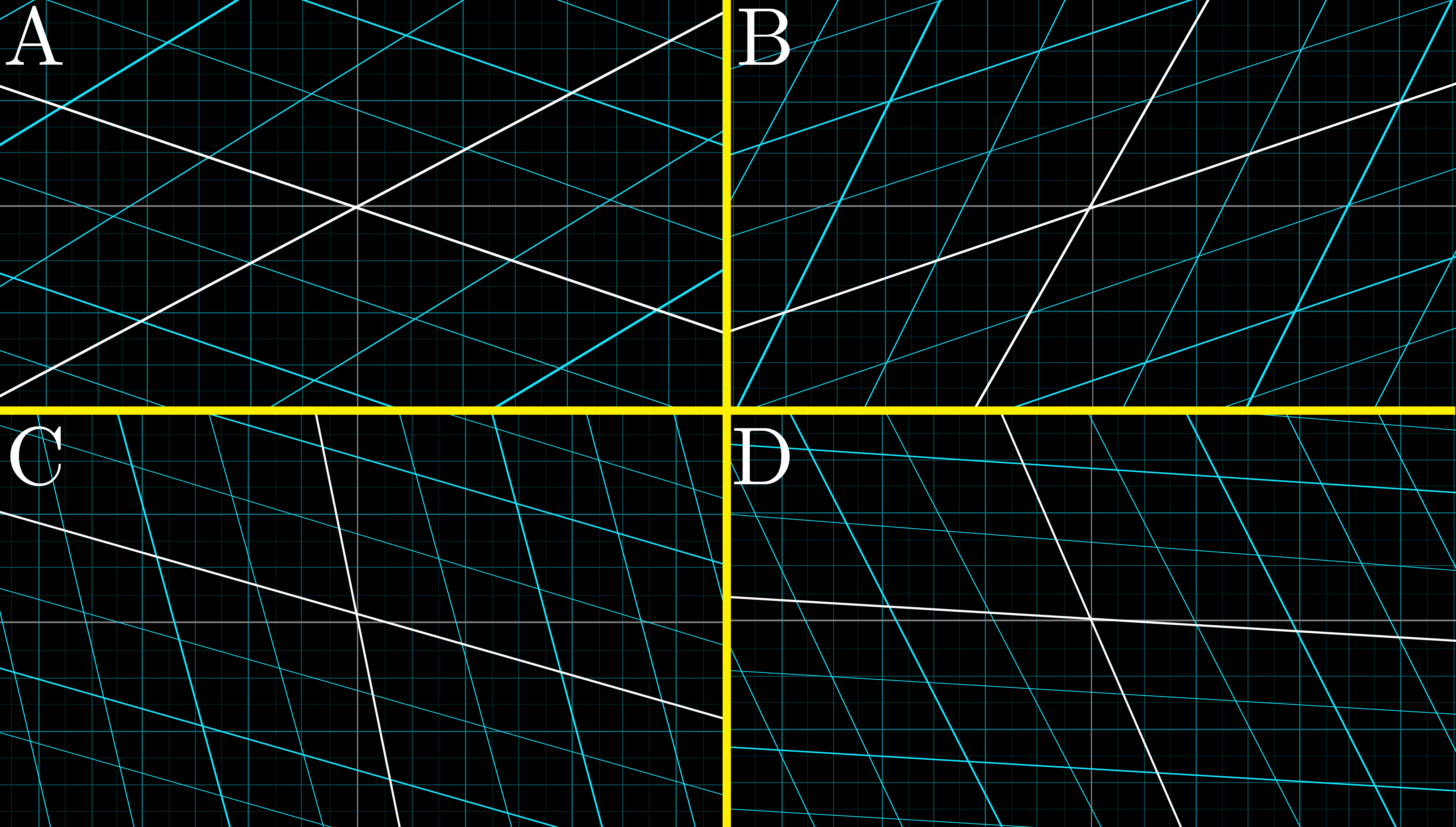
Which of the transformations in the following image match the given matrix?

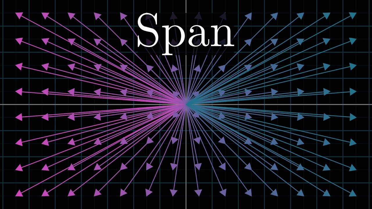
Linearly Dependent Columns

If the vectors that $\hat{\imath}$ and $\hat{\jmath}$ land on are linearly dependent, which if you recall from the last chapter means one is a scaled version of the other, it means the linear transformation squishes all of 2D space onto the line where those vectors sit. This is also known as the one-dimensional span of these two linearly dependent vectors.

Formal Properties

TODO: move formal properties here

As you can imagine, there's an unimaginably huge number of possible transformations, most of which would be rather complicated to think about. Luckily, linear algebra limits itself to a special type of transformation that's easier to understand: Linear transformations.

Let's start with the algebraic definition of linearity, then see what it looks like visually. A transformation $L$ is linear if it satisfies the following two properties.

\begin{align*} \text{$L$ preserves sums:} \qquad L( {\color{green}\overrightarrow{\mathbf{v}}} + {\color{blue}\overrightarrow{\mathbf{w}}} ) &= L({\color{green}\overrightarrow{\mathbf{v}}}) + L({\color{blue}\overrightarrow{\mathbf{w}}}) \\\\ \text{$L$ preserves scaling:} \qquad L( s{\color{green}\overrightarrow{\mathbf{v}}} ) &= sL({\color{green}\overrightarrow{\mathbf{v}}}) \end{align*}

To help appreciate just how constraining these two properties are, and to reason about what this implies a linear transformation must look like, consider the important fact from the last chapter that when you write down a vector with coordinates, say $\overrightarrow{\mathbf{v}} = \begin{bmatrix}-1\\2\end{bmatrix}$ , you are effectively writing it as a linear combination of two basis vectors. In this case,

\overrightarrow{\mathbf{v}} = -1{\color{green} \hat{\imath}} + 2{\color{red} \hat{\jmath}}.

What it looks like for a transformation to be linear is that after the transformation, the transformed version of $\overrightarrow{\mathbf{v}}$ will be this same linear combination of the transformed versions of ${\color{green} \hat{\imath}}$ and ${\color{red} \hat{\jmath}}$ .

Why? This pops out of what we mean when a linear transformation preserves both sums and scalar products.

\begin{align*} L\left(-1{\color{green} \hat{\imath}} + 2{\color{red} \hat{\jmath}} \right) &= L(-1{\color{green} \hat{\imath}}) + L(2{\color{red} \hat{\jmath}}) \\ &= -1 \cdot L({\color{green} \hat{\imath}}) + 2 \cdot L({\color{red} \hat{\jmath}}) \end{align*}

This means linearity is incredibly restrictive. If you know where the two basis vectors $\color{green} \hat{\imath}$ and $\color{red} \hat{\jmath}$ go, everything else will follow!

Visually, this means the entire grid of 2d points "follows along" with $\color{green} \hat{\imath}$ and $\color{red} \hat{\jmath}$ , so to speak. You can know that a transformation is linear if all those grid lines which began parallel and evenly spaced remain parallel and evenly spaced (why?). Actually, it's a tiny bit more constrained that that. If a transformation is linear, it must also fix the origin in place (again, why?).

To give just one important example of a linear traformation, consider rotation about the origin. Notice how all the grid lines remain parallel and evenly spaced.

However, for most other linear transformations, grid lines which started off perpendicular to each other may not stay perpendicular. It is perfectly allowable, and in fact much more common, for there to be some shearing effect.

Who cares

The reason linear algebra is so important is that linear functions come up all the time throughout science and engineering. Sometimes this conception of them as transformations is very literal, as in the case of a computer graphics programmer trying to describe rotation in space. More often, a linear function arises in a less directly visual context, say as one step in a neural network, but being able to visualize it helps to glean some insight into how to think about it.

Conclusion

Understanding how matrices can be thought of as transformation is a powerful mental tool for understanding the various constructs and definitions concerning matrices, which we'll explore as the series continues. This includes the ideas of matrix multiplication, determinants, how to solve systems of equations, what eigenvalues are, and much more. In all these cases, holding the picture of a linear transformation in your head can make the computations much more understandable.

On the flip side, there are cases where you may want to actually describe manipulations of space; again graphics programmings offers a wealth of examples. In those cases, knowing that matrices give a way to describe these transformations symbolically, in a manner conducive to concrete computations, is exceedingly helpful.

Enjoy this lesson? Consider sharing it.

Twitter Reddit Facebook

Want more math in your life?

Notice a mistake? Submit a correction on GitHub

Linear combinations, span, and basis vectors

Matrix multiplication as composition

Table of Contents