Chapter 5Three-dimensional linear transformations

Lisa: Well, where's my dad?

Frink: Well, it should be obvious to even the most dimwitted individual who holds an advanced degree in hyperbolic topology that Homer Simpson has stumbled into... dramatic pause... the third dimension.

Here's a quick footnote between chapters.

In the last two chapters, we talked about linear transformations and matrices, but only showed the specific case of transformations that take two-dimensional vectors to other two-dimensional vectors. Throughout this series we will work mainly in two-dimensions, mostly because it's easier to actually see on the screen and wrap your mind around. And more importantly, once you get all the core ideas in two dimensions, they carry over pretty seamlessly to higher dimensions.

Nevertheless it's good to peek our head outside of flatland now and then to see what it means to apply these ideas to more dimensions.

Three-dimensions

For example, consider a linear transformation with three-dimensional vectors as inputs and three-dimensional vectors as outputs.

We can visualize this by smooshing around all the points of three-dimensional space, as represented by a grid, in such a way that keeps grid lines parallel and evenly spaced.

Just as with two dimensional space, every point of space that we see moving around is really just a proxy for the vector who has its tip at that point, and what we're really doing is thinking about input vectors moving to their corresponding outputs.

And just as with two dimensions, one of these transformations is completely determined by where the basis vectors go. But now, there are three basis vectors: The unit vector in the x direction, i hat, the unit vector in the y direction, j hat, and the unit vector in the z direction, called k hat.

In fact it's easier to think about these transformations by only following the basis vectors, since the full 3d grid representing all points can get messy. By leaving a copy of the original axes in the background, we can think about the coordinates where each of the three basis vectors lands.

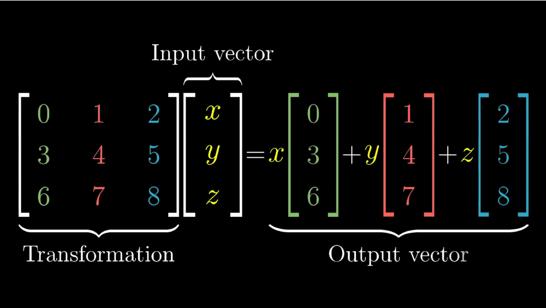
Record the coordinates of these three resulting vectors as the columns of a 3x3 matrix. This gives a matrix that completely describes your transformation using 9 numbers.

As a simple example, consider the transformation here that rotate space 90 degrees around the y axis.

It takes i hat to the coordinates [0, 0, -1], so that's the first column of our matrix. It doesn't move j hat, so the second column is [0, 1, 0]. And it moves k hat onto the x axis at [1, 0, 0], so that becomes the third column of our matrix.

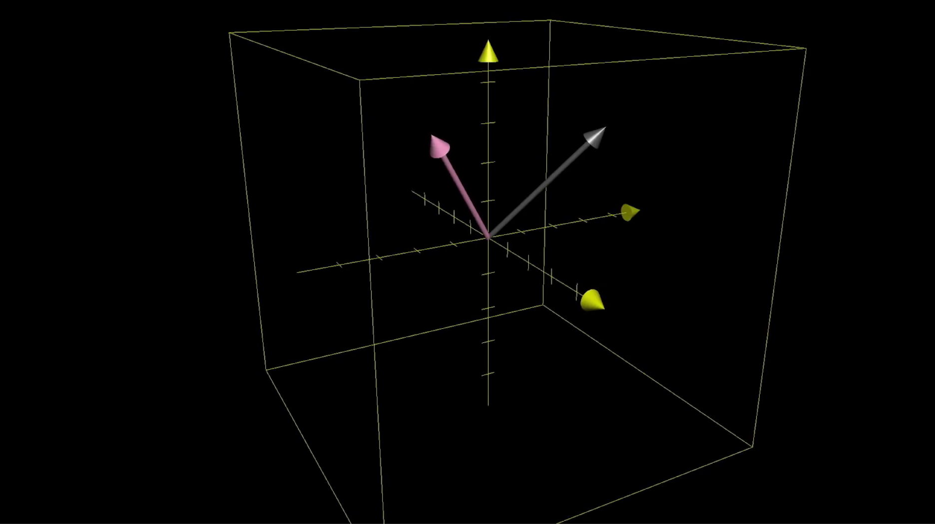
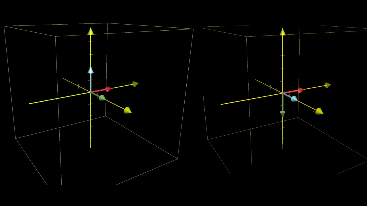
To see where a vector with coordinates $x$, $y$ and $z$ lands, the reasoning is almost identical to what it was for two dimensions: Each of those coordinates can be thought of as instructions for how to scale each basis vector, so that they add together to get your vector.

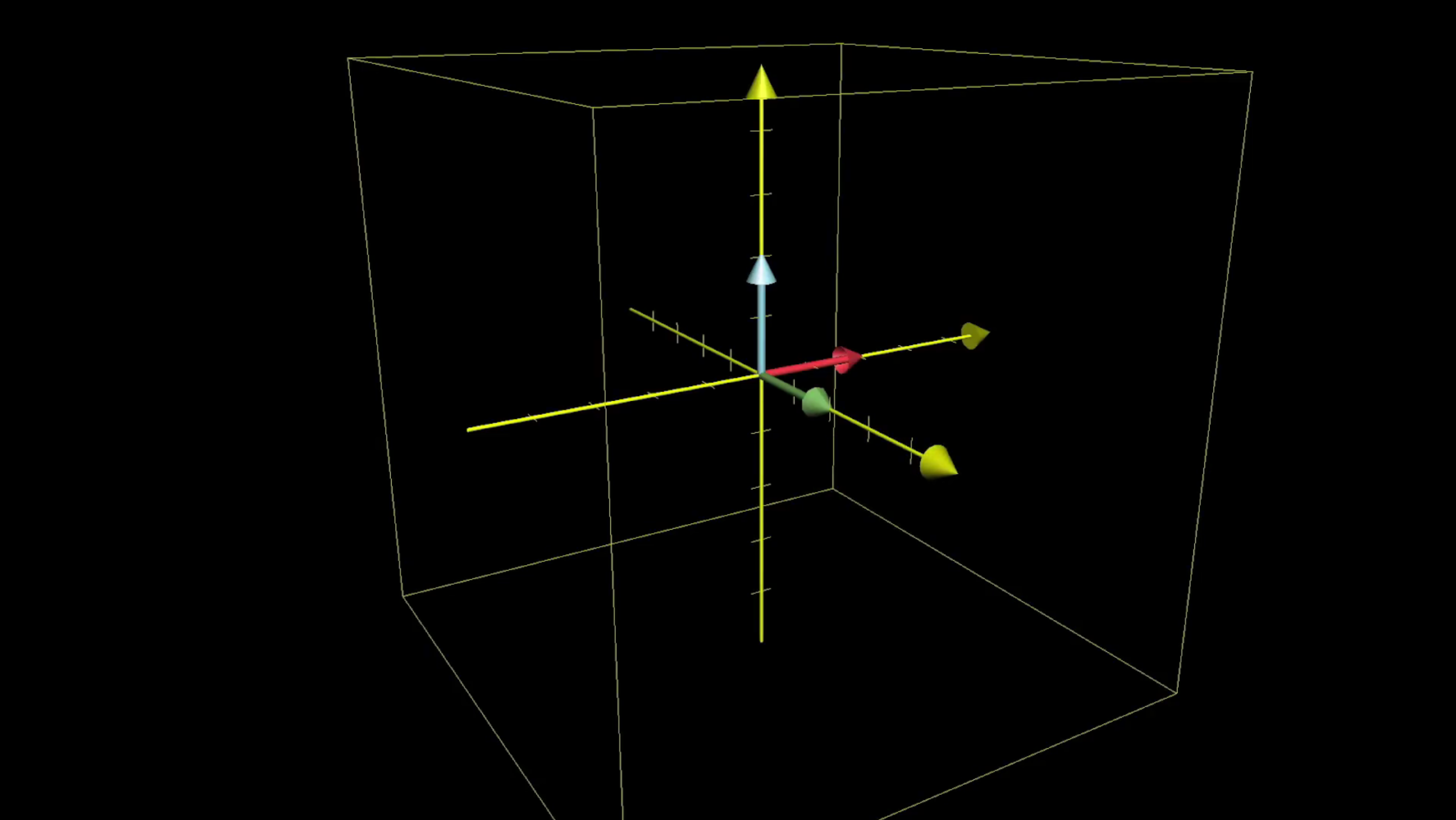
And the important part, just like the 2d case, is that this scaling and adding process works both before and after the transformation. Note how the axis are tilted in the following image:

So to see where your vector lands, you multiply those coordinates by the corresponding column of the matrix, and add together the three results.

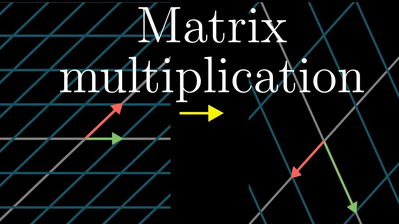
Multiplying two matrices is also similar: Whenever you see two 3x3 matrices getting multiplied together, you should imagine first applying the transformation encoded by the right one, then applying the transformation encoded by the left one.

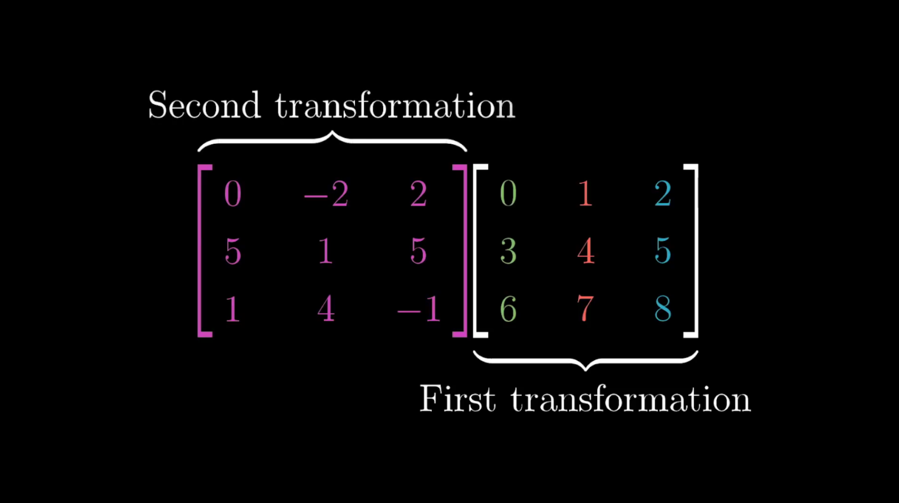
3d matrix multiplication turns out to be very important for computer graphics and robotics, since things like rotations in three-dimensions can be very hard to describe, but are easier to wrap your mind around if you break them down as the composition of different transformations.

TODO: redraw 3D transformations using just basis vectors

Performing this matrix multiplication numerically is, once again, very analogous to the two-dimensional case. In fact, a good way to test your understanding of the last chapter would be to reason through what specifically it should look like, thinking closely about how it relates to the idea of applying two successive transformations of space.

Puzzle

Here's another puzzle for you: It's also meaningful to talk about a linear transformation from two-dimensional space to three-dimensional space, or from three-dimensions down to two. Can you visualize such a transformations? And can you represent them with matrices? How many rows and columns for each one? When is it meaningful to talk about multiplying such matrices, and why?